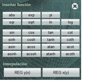
 To open the function keyboard, click on the f (x) link that is located on the equation editor when we position ourselves on it.
In the lower section of the function keyboard, there are two interpolation buttons that allow you to obtain linear interpolation results in the connected curve. These generic variables perform not only the interpolation in the curve but also perform the uncertainty estimation of it, integrating its contribution to the model.
It is important to understand that this calculation does not represent what is usually done when we do it manually, but it integrates all the tools available in the simulation of the model, as well as the data obtained during the simulation of the connected curve.
REG_y (x). Interpolates the observed response ( y ) of an indicated value from x axis, estimating its associated total uncertainty. The value of x can be numerical, a variable or even part of the model equation. For example REG_y (5), REG_y (A) or REG_y (coef_a * ABS (A1-A2)).
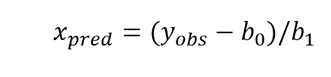
REG_x (y). Given a value, variable or fragment of the equation corresponding to y axis, interpolate and estimate the associated uncertainty of the corresponding value of x .
Uncertainty of interpolation.
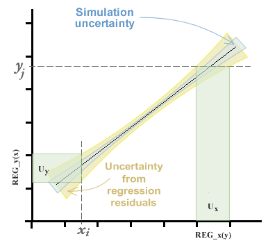
In the chapter on Using the calibration curve panel we saw that we could estimate the curve of best fit by the method of ordinary, inverse and total least squares (the latter by means of the method of analysis of the primary component). Whichever method is chosen, we will obtain coefficients of the equation of the line, in addition to a range of variable uncertainty along the curve, composed of the uncertainty of simulation and that contributed by the variance of the residuals. This topic can be seen in more depth in the chapter of regressions and curves .
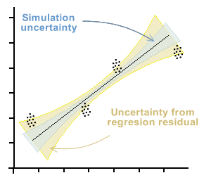
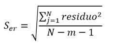
The uncertainty in the interpolation, then, will be given by the standard error of the curve in the axis from which it intends to interpolate.
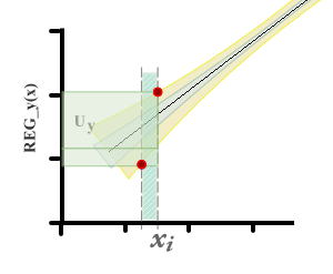
It can be seen that there are two differences with respect to the method that is usually used to estimate uncertainty in calibration curves. First, zero uncertainty is not expected on the x axis.
On the other hand, when you want to estimate the value of x i from a y i observed, the uncertainty interval in x is taken from the residual variance in x . In the graphs you can see a representation of the uncertainty of the measurand in each case.
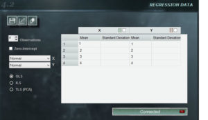 The regression panel of MCM Infinite Alchimia allows great flexibility when constructing a calibration curve for our test model.
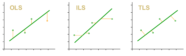
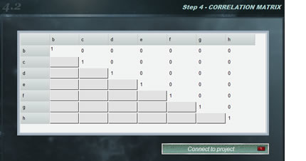 Frequently test models are used that contain two or more magnitudes with some degree of correlation, that is, that systematically, when modifying the value of one of them, the other increases or decreases. The correlation coefficients between two variables vary between -1 and 1, where the value indicates the strength of the correlation, while the sign indicates the direction. In this way, we understand that if the correlation is = 1 there is an absolute direct proportionality between the magnitudes whereas if the value is -1 the proportionality is inverse. On the other hand, a zero value for the correlation coefficient indicates that the variables are independent.
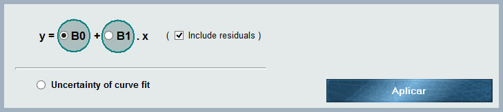
 This distribution is not a distribution in itself, but a powerful and exclusive form of MCM Alchimia to enter raw values of repeatability to the model of our trial without having to make any kind of previous operations in a spreadsheet.
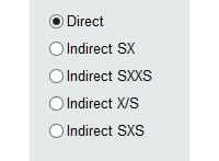 To the left of the panel we have 5 radio buttons (selectors), which will indicate to the software the form in which the input data will be entered. We will then have 5 input forms:
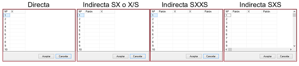
 This section of the panel provides two ways to perform the simulation from the parameters of the previously defined distribution from the entered values:
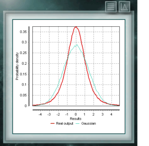 It is usual to assume in all types of analyzes, tests or calibrations, that repetitive events without external stimuli that vary their probabilities, will be distributed according to a normal or gaussian distribution defined by the mean and the standard deviation calculated for the sample. Strictly speaking this is only true when the number of repetitions is large, consistent with the central limit theorem, however when we do not have enough information to describe the properties of this gaussian distribution because our study sample is not large enough, suppose that these conditions are also fulfilled, we will surely throw values of uncertainty underestimated for our measurement, as indicated in the guide JCGM 100 – Guide to the expression of uncertainty in measurement.
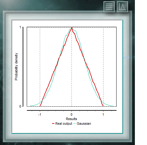 The continuous triangular distribution is characterized by being bounded to two extremes as in the case of the rectangular, but also has a mode (or value more probabe) within that range. The probability in any subinterval of equal length will increase linearly until fashion and then descend in the same way to the upper bound. This distribution is widely used in variables where information is limited, as in the case of the uniform, but where we have an approximate knowledge of the Modal value, that is, where, although the exact point of this value is not known, has information of the region or subinterval where to find it.
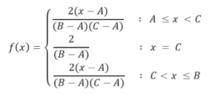
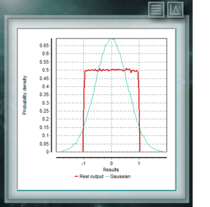 This continuous distribution is characterized by having the same probability for any value of the interval. It is widely used for contributions of type B uncertainties in which only the major and minor dimensions of the interval are known, for example in the division or resolution of a digital instrument. In many cases this distribution can also be assigned when there is little information about the random variable, in bibliographic data or when the coverage factor of an uncertainty is not known,