
 It is usual to assume in all types of analyzes, tests or calibrations, that repetitive events without external stimuli that vary their probabilities, will be distributed according to a normal or gaussian distribution defined by the mean and the standard deviation calculated for the sample. Strictly speaking this is only true when the number of repetitions is large, consistent with the central limit theorem, however when we do not have enough information to describe the properties of this gaussian distribution because our study sample is not large enough, suppose that these conditions are also fulfilled, we will surely throw values of uncertainty underestimated for our measurement, as indicated in the guide JCGM 100 – Guide to the expression of uncertainty in measurement.
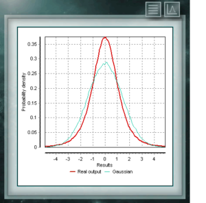
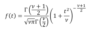
This same problem was raised by William Gosset, who signed his work as “Student” for reasons of business confidentiality of the company where he worked. Gosset needed to estimate, from experimental data, a distribution that represented small samples of unknown variance. This distribution function proposed by Gosset is known as Student t distribution, and responds to the following general equation:
In any normally distributed population, the Student t distribution allows increasing the width of the resulting normal distribution to increase the uncertainty associated with the measurand as a result of the poverty of information provided by a small sample on the total lot. To the extent that this sample is larger, the distribution t will approach the Normal obtained from the standard deviation of the sample until it is identical to this latter for infinite repetitions of the event.
The correct thing in all types of analysis is to assign to repetitive events the distribution t with a parameter gl, which will be the degrees of freedom, whose value will be the number of repetitions minus 1. MCM Alchimia allows to simulate a random sample according with the Student t distribution, not only with this parameter of form (degrees of freedom), but with parameters of scale and position, through the standard deviation and the mean respectively, so that it can be used in any situation where appropriate, with no additional operations.
Input parameters:
- Mean value. This parameter defines the displacement of the function on the abscissa axis. Corresponds to the average value, or average, of the random variable. The data collection of this variable, therefore, will be distributed on both sides of this function. In the case of this distribution, as in all symmetrical functions, the average will coincide with statistical Mode.
- Degrees of freedom. Corresponds to the number of repetitions minus 1, Represents the number of values that can vary without modifying the value of the sample mean.
- Standard deviation. Measure of the dispersion of the values with respect to the sample mean. If this distribution is used for Type A (statistical) uncertainty components, this value can be calculated according to the equation:
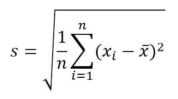
where n is the number of values or repetitions. On the other hand, if what you want to know is the standard deviation of the sample means, this value can be obtained by dividing s / √ n .
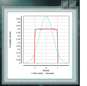
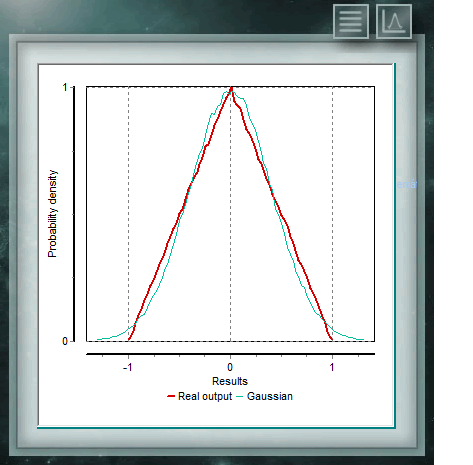 The continuous triangular distribution is characterized by being bounded to two extremes as in the case of the rectangular, but also has a mode (or value more probabe) within that range. The probability in any subinterval of equal length will increase linearly until fashion and then descend in the same way to the upper bound. This distribution is widely used in variables where information is limited, as in the case of the uniform, but where we have an approximate knowledge of the Modal value, that is, where, although the exact point of this value is not known, has information of the region or subinterval where to find it.
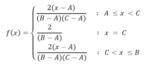
 This continuous distribution is characterized by having the same probability for any value of the interval. It is widely used for contributions of type B uncertainties in which only the major and minor dimensions of the interval are known, for example in the division or resolution of a digital instrument. In many cases this distribution can also be assigned when there is little information about the random variable, in bibliographic data or when the coverage factor of an uncertainty is not known,
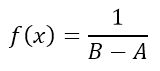
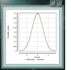 This distribution is the one that most frequently is representing natural and social events. Much of the evidence from classical statistics, as well as the estimation of uncertainties, is based on the assumption that the data conform to a normal distribution. From the theoretical perspective, the Central Limit Theorem maintains that given a random sample of sufficiently large size, it will be observed that the distribution of means follows an approximately normal distribution. The general formula of this distribution is:
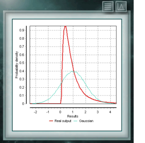 This distribution represents random variables whose logarithms are distributed according to a normal distribution. The lognormal distribution takes different forms depending on the value of its scale parameter and is often used in the reliability of high technology products and also in microbiological counts since they are based on the multiplicative growth model.
 This continuous probability distribution in the field of positive reals is intimately related to the Normal distribution, for example, it is the sample distribution of σ². The Xi (or Chi) Square distribution is defined with a single parameter which are degrees of freedom. The function is always asymmetric and biased to the right. This distribution is very frequently used in various branches of science since it allows analyzing data sets and determining if the difference between them is due to chance (null hypothesis) or to another external factor.
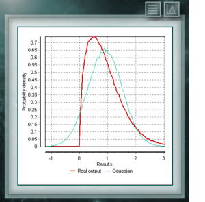 This distribution is a continuous function in the domain of positive real numbers, frequently used in economics, meteorology and telecommunications, as well as other specific applications, such as the reliability rate or the survival of organisms or machines. The random variables that have the Weibull distribution model the distribution of faults in systems when the fault ratio is proportionally related to a power of time. This distribution is defined from a characteristic Form (> 0) parameter that would indicate the failure rate, so that if the failure rate decreases, it is constant or increases with time. That corresponds with if the parameter k is smaller, equal or greater than 1.
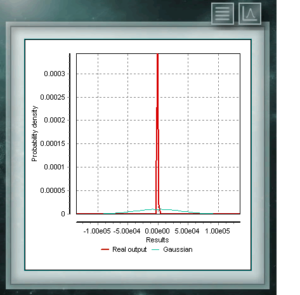 The Cauchy distribution has the particularity of being of the Gaussian type of distributions, however it has the highest peak and the tails decompose very slowly. Although MCM Alchimia suitably generates the pseudo-random samples for this distribution, the results graph will look like an isolated peak since the abscissa axis of it is taken in the 99% coverage probability interval. Because the decay of the tails is so gradual, the range of significant probabilities becomes very narrow.
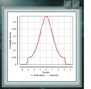 The distribution of Von Mises is a continuous function of the circular calls, that is, they are defined for the real ones in the interval from 0 to 2p. This function is currently used preferably in the field of epidemiology to describe the spread of diseases or technological applications such as signal processing. The Von Mises distribution is also known as normal circular as it is similar to Gaussian, but restricted to the circular plane.