
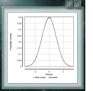
 This distribution is the one that most frequently is representing natural and social events. Much of the evidence from classical statistics, as well as the estimation of uncertainties, is based on the assumption that the data conform to a normal distribution. From the theoretical perspective, the Central Limit Theorem maintains that given a random sample of sufficiently large size, it will be observed that the distribution of means follows an approximately normal distribution. The general formula of this distribution is:
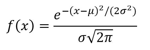
where μ represents the location and σ the scale of the function. In order to estimate a measurement uncertainty, μ corresponds to the mean and mode value of the random variable, while σ is the standard deviation.
Input parameters:
- Mean. Average value, or average of the random variable. The data collection of this variable, therefore, will be distributed on both sides of this function. In the case of this Normal or Gaussian distribution, the mean will coincide with fashion.
- Standard deviation. Measure of the dispersion of the values with respect to the sample mean. If this distribution is used for Type A (statistical) uncertainty components, this value can be calculated according to the equation:
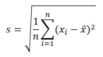
where n is the number of values or repetitions. On the other hand, if what you want to know is the standard deviation of the sample’s mean, this value can be obtained by dividing s / √ n .
If the parameter to which this distribution is assigned corresponds to the uncertainty contribution from a calibration certificate, the standard deviation corresponds to the standard uncertainty ( u ), or to the expanded uncertainty divided by the coverage factor k.
More help
 This distribution represents random variables whose logarithms are distributed according to a normal distribution. The lognormal distribution takes different forms depending on the value of its scale parameter and is often used in the reliability of high technology products and also in microbiological counts since they are based on the multiplicative growth model.
 This continuous probability distribution in the field of positive reals is intimately related to the Normal distribution, for example, it is the sample distribution of σ². The Xi (or Chi) Square distribution is defined with a single parameter which are degrees of freedom. The function is always asymmetric and biased to the right. This distribution is very frequently used in various branches of science since it allows analyzing data sets and determining if the difference between them is due to chance (null hypothesis) or to another external factor.
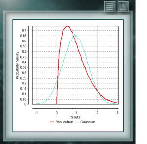 This distribution is a continuous function in the domain of positive real numbers, frequently used in economics, meteorology and telecommunications, as well as other specific applications, such as the reliability rate or the survival of organisms or machines. The random variables that have the Weibull distribution model the distribution of faults in systems when the fault ratio is proportionally related to a power of time. This distribution is defined from a characteristic Form (> 0) parameter that would indicate the failure rate, so that if the failure rate decreases, it is constant or increases with time. That corresponds with if the parameter k is smaller, equal or greater than 1.
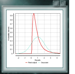
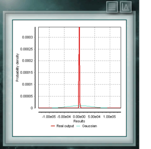 The Cauchy distribution has the particularity of being of the Gaussian type of distributions, however it has the highest peak and the tails decompose very slowly. Although MCM Alchimia suitably generates the pseudo-random samples for this distribution, the results graph will look like an isolated peak since the abscissa axis of it is taken in the 99% coverage probability interval. Because the decay of the tails is so gradual, the range of significant probabilities becomes very narrow.
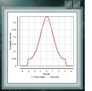 The distribution of Von Mises is a continuous function of the circular calls, that is, they are defined for the real ones in the interval from 0 to 2p. This function is currently used preferably in the field of epidemiology to describe the spread of diseases or technological applications such as signal processing. The Von Mises distribution is also known as normal circular as it is similar to Gaussian, but restricted to the circular plane.
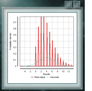 The NegBinomial distribution is discrete distribution, defined in the domain of positive integers. It is similar to the binomial distribution except that the n parameter refers to non-total and incomplete events. In other words, a random variable with NegBinomial distribution of parameters n and p represents the number of successes whose probability is p, which are achieved in a sequence of n failed trials. The parameters by means of which this distribution is defined have the same form as those that represent the Binomial distribution, although, as we said, the parameter n represents a different quality.
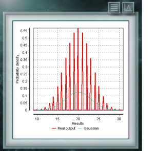 Dies ist eine diskrete Verteilung, deren Domäne die Menge positiver Ganzzahlen ist, die die Anzahl der in einer Folge von n Versuchen erzielten Erfolge darstellt. Diese Tests müssen dichotom sein, dh sie bieten nur zwei Möglichkeiten (Erfolg und Misserfolg) und haben eine definierte Erfolgswahrscheinlichkeit = p.
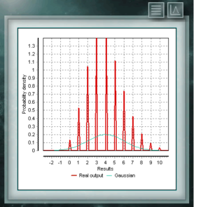 The Poisson distribution is a discrete distribution defined for the domain of integers greater than zero. It is used mostly to represent the probability that a certain number of events will occur in a period of time, a defined distance, area, volume, etc.,
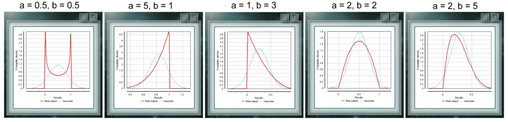 This distribution is a continuous function with two parameters which must take real values greater than zero. The function is defined between 0 and 1. A particular case of the Beta distribution is when both form parameters take values = 1. In this case the function will coincide with a uniform distribution.